Is 99% of your System’s Latency due to Accidental Complexity?

In the realm of frequency trading and other latency-sensitive trading strategies, even a few additional microseconds can determine whether a trade lands ahead of, or behind, the competition. When your trading infrastructure must digest vast quantities of real time market data, route data packets through multiple layer switches, and respond to matching engines at the lowest latency possible, accidental complexity can silently erode performance and profitability.

In this article we will look at a real life example of accidental complexity in the context of latency to help explain what it is, and will provide a strategy for how to investigate how you can reduce potential accidental complexity and increase your system’s performance.

Along the way, we will reference common components of contemporary trading systems—such as access layer switches, mid layer devices in a data center, and colo entry switches deployed at exchanges like Deutsche Börse or any major stock exchange—to show how hidden delays creep into real time trading workflows.

Essential vs Accidental Complexity

Firstly, as the two are often confused, let’s clarify the difference between essential and accidental complexity:

Essential complexity is inherent in the problem that is being solved, the complexity we can’t avoid as it is part of what the software is aiming to address, e.g. the time it takes to send an event from A to B or for a matching engine to process an incoming tick trade.

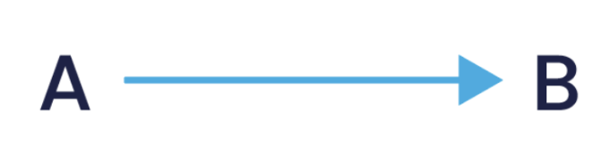
Accidental complexity is the complexity that is not inherent in the problem, but rather in the solution. This is the complexity that is not fundamental and can be removed or reduced with a better design or technology choice. In latency trading systems this often manifests as unnecessary object allocations, excessive network hops across the access layer, or verbose market data processing pipelines that bloat each data packet with metadata that is never used downstream.

Real-Life Example of Accidental Complexity

If we look at getting from St. Paul’s Cathedral to Shakespeare’s Globe in London in two different ways we can grasp what accidental complexity is all about.

Driving requires an indirect route, and has parking challenges in both places. For market participants, this is analogous to routing an order through multiple mid layer switches in a crowded data center, each hop adding latency characteristics that are not essential to the trading objective:

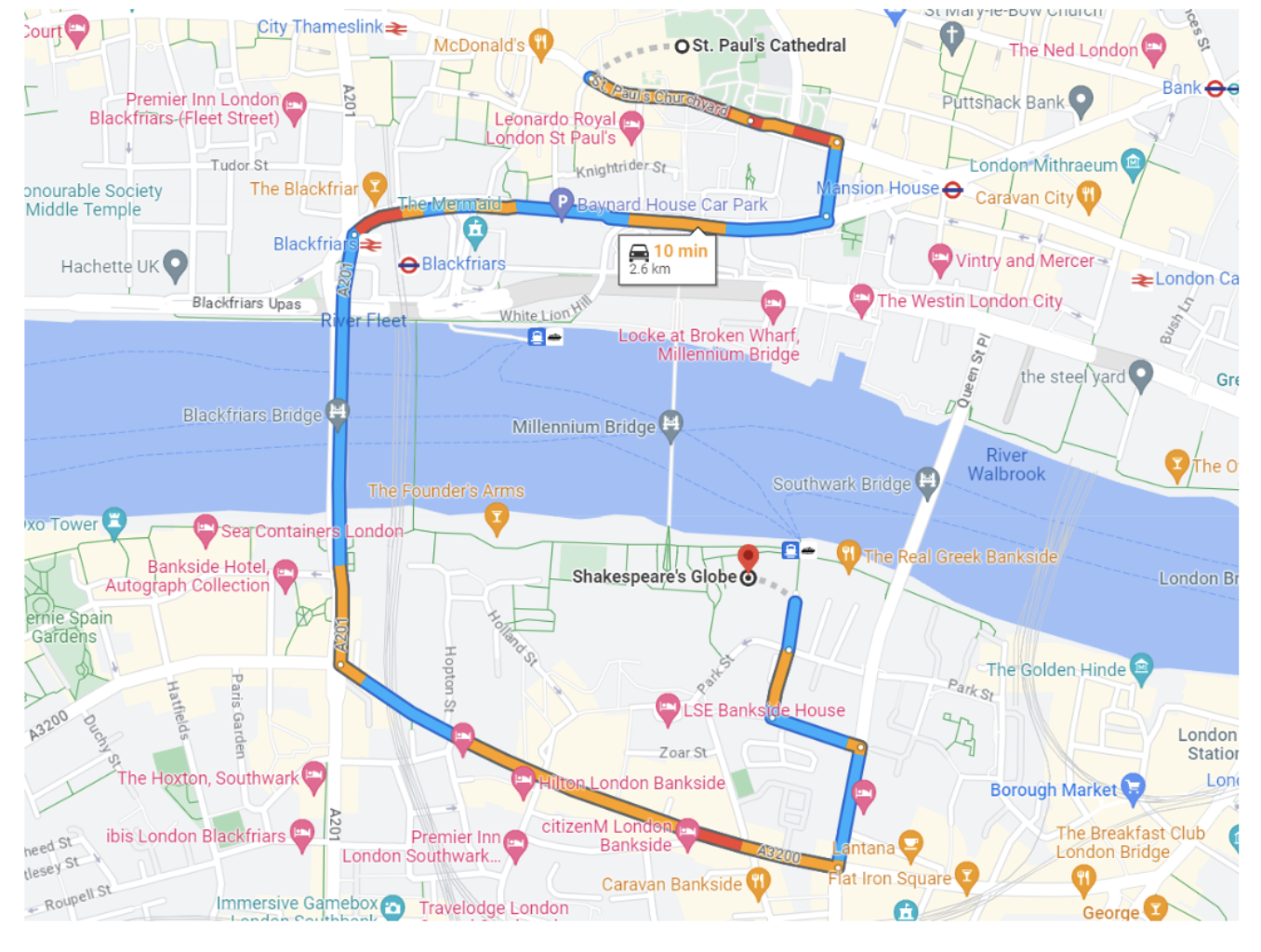
Image 1. Driving from St. Paul’s Cathedral to Shakespeare’s Globe in London

Walking on the other hand offers a more direct route, and hence minimises accidental complexity. Similarly, a direct fibre cross-connect within a refresh colo environment can bypass non-essential routing gear, ensuring the lowest latency path between your access layer switch and the exchange’s matching engine:

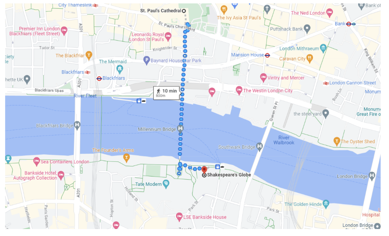
Image 2. Walking from St. Paul’s Cathedral to Shakespeare’s Globe in London

Visualising Accidental Complexity in Low Latency Systems

In the previous example it was easy to grasp accidental complexity, but in the realms of low-latency systems, where latencies are invisible, it can be more difficult to understand. One way to make latencies more tangible would be to translate latencies into distances.

For instance, Kafka’s 99th percentile latency in a round-trip benchmark that took 2.6 milliseconds is the equivalent of sending a signal from New Haven to Washington, which is 330 miles. For a trading desk processing EOBI market data or streaming futures contracts, 2.6 milliseconds could be the difference between capturing the spread and missing the book entirely:

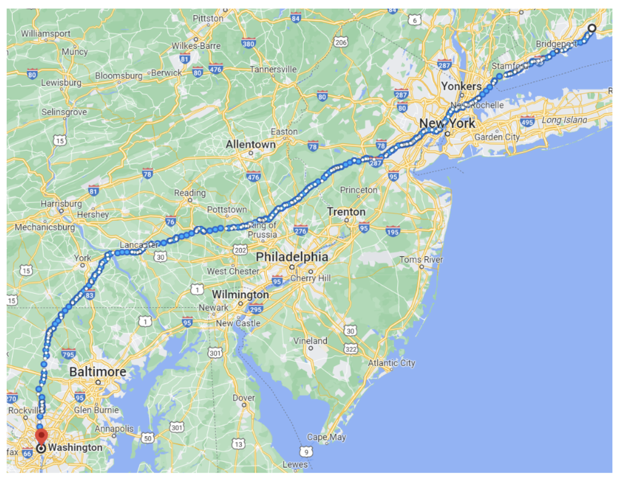
Image 3. RTT client to microservice via Kafka, 2.6ms or 330 miles

Reviewing the client Kafka’s allocation rate we found a substantial amount of garbage collection occurring, with Flight Recorder showing an allocation rate of about 6.5 GB per second. This level is normal for most Java applications, but it’s not essential and must be avoided when pursuing the lowest possible latencies, especially for latency algorithmic trading where a single GC pause can derail the execution of a sophisticated trading strategy.

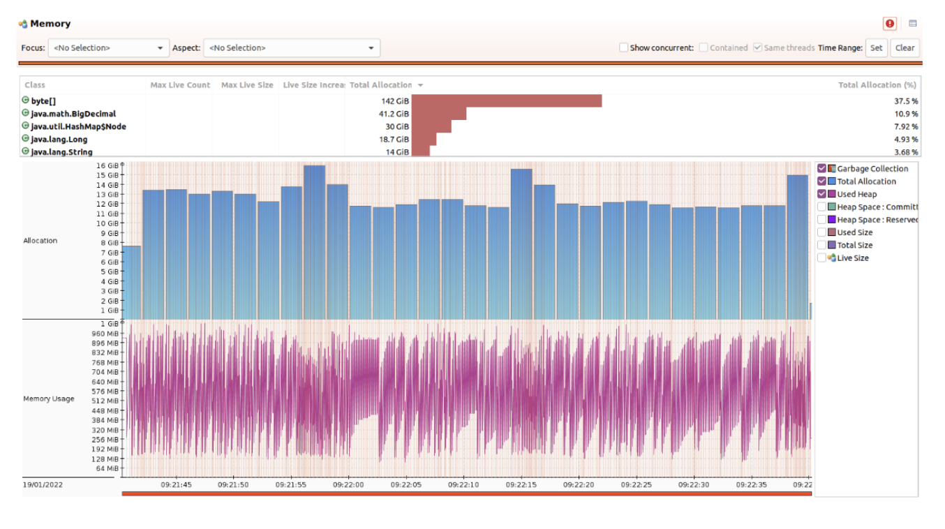
Image 4. Memory Usage in Kafka

On the other hand, using Chronicle Queue for the same benchmark, the 99th percentile latency was just 3.67 microseconds – almost 700 times less, and the equivalent of sending a signal across Battery Park. For electronic trading firms striving for sub-10 µs round-trip between an order gateway and the exchange, this is transformational:

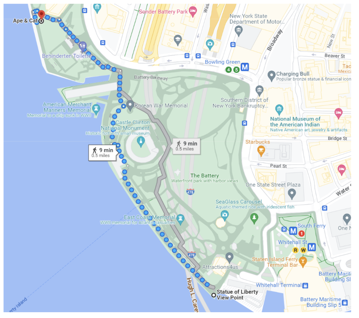
Image 5. RTT via Chronicle Queue, 0.003ms or 800 yards

When looking into the allocation rate with Chronicle Queue, it highlighted that most of the garbage was due to Java 8’s Flight Recorder. With Java 17’s Flight Recorder this was dramatically reduced, freeing precious CPU cycles for real time market data processing and accelerating response to ETI responses from venues such as Deutsche Börse:

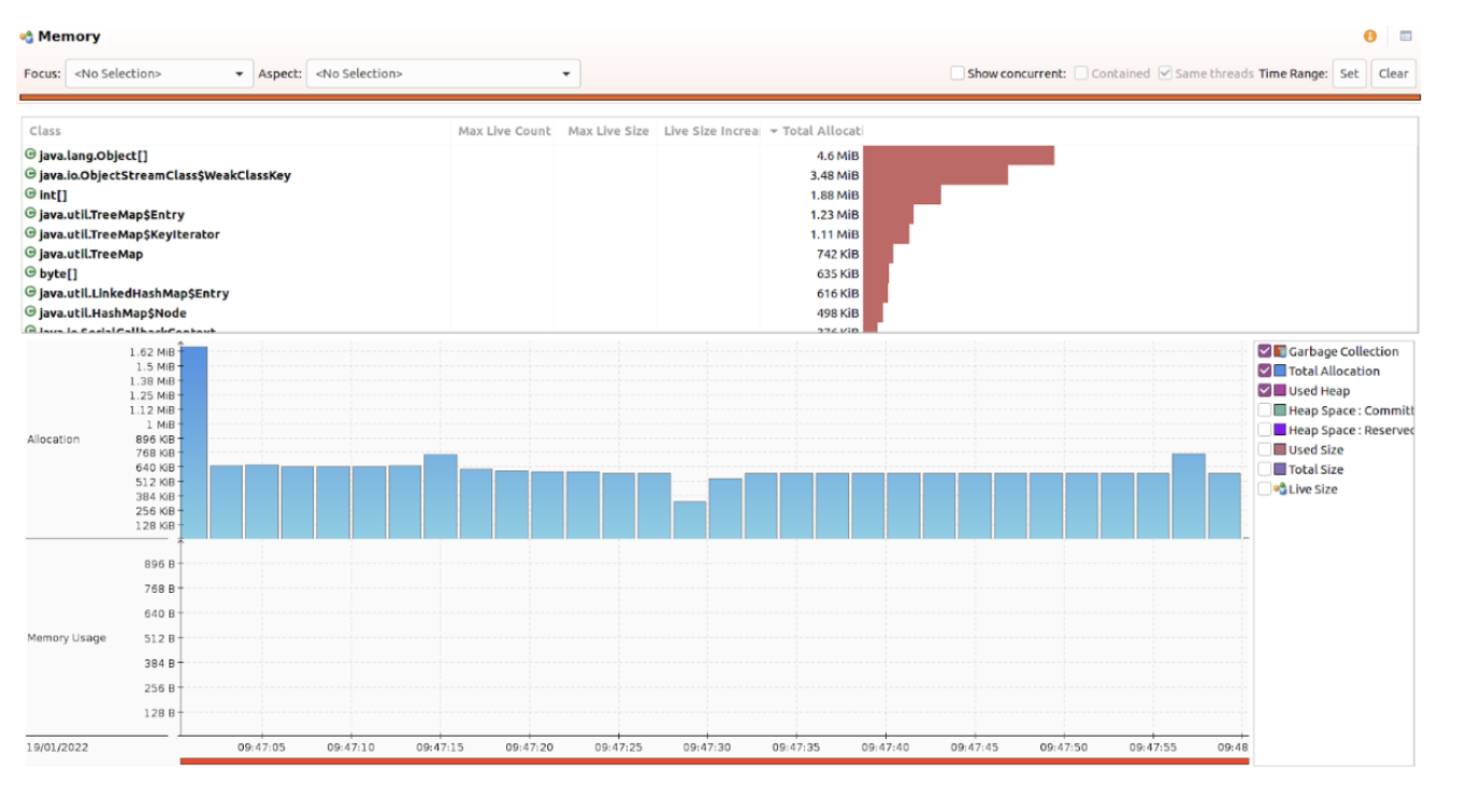
Image 6. Memory Usage in Chronicle Queue

Accidental Complexity in Chronicle Queue

In Image 7 we can see that open source Chronicle Queue in Java still has some accidental complexity in the higher percentiles. Meanwhile, there are commercial C++ and Rust versions, and these have much more consistent latencies, making them attractive for firms pursuing latency electronic trading or high-velocity tick trade capture across multiple stock exchanges:

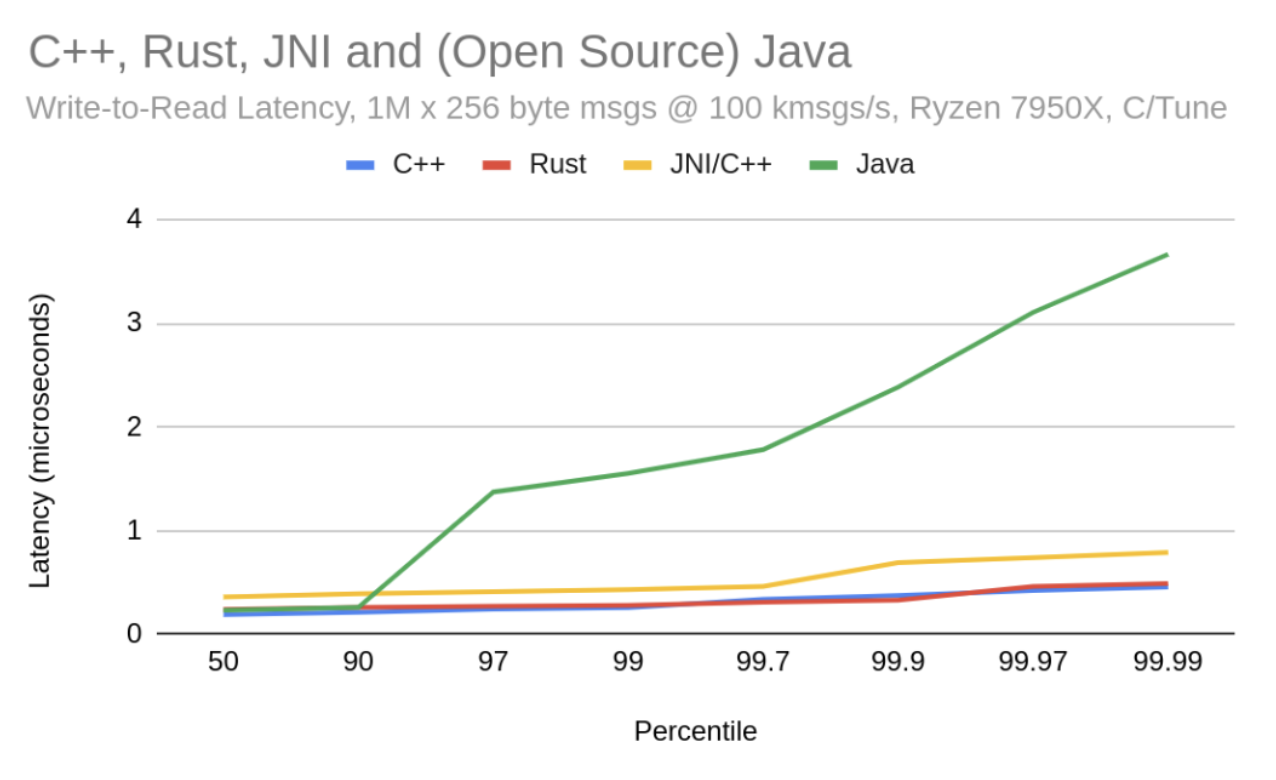
Image 7. Chronicle Queue Enterprise, Chronicle Queue Open Source, Multi Language

99% Accidental Complexity

Back to the latency comparison from earlier; as Chronicle Queue was 700 times faster – or that the same task could be completed in 1% of the time – it indicated that 99% of the latency was accidental, for the purposes of this benchmark.

Determining the amount of accidental complexity in a system is challenging, but a comparison between different strategies can provide some indication. Ultimately, any differences in completing the same tasks could be considered ‘accidental’. It is also worth noting that just because one strategy may be faster, it does not inherently mean that there is not further, or different accidental complexity in that too. For example, a tech refresh that swaps older mid layer switches for the latest access layer devices may lower latency now, yet still leave hidden bottlenecks in a precision timestamp file pipeline or in the PS gateway used to stamp every market data packet.

If you are interested in finding out how your system’s latency could be reduced by investigating potential accidental latency, book a demo with our experts, or find out more on our website. Whether you are optimising a futures contracts arbitrage strategy, refining a high-frequency trading system, or simply seeking a cleaner network topology inside your colo entry switches, our team can guide you towards measurable performance gains.